Dynamic Range, Exposure And Tonemapping

I want to try to talk about the intuition behind exposure and tonemapping as they’ve been showing up a lot for me, and dealing with luminance is a good introduction to some interesting post processing techniques used in recent games, such as automatic exposure, temporal adaption, and local tonemapping.

Dynamic Range

Dynamic range example

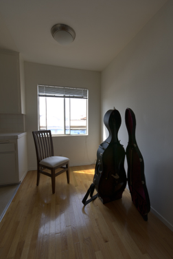
Example from Hable’s 2010 GDC talk. Note the lack of detail in the cello and window; they are clipped to a solid blob of black and white respectively.

As part of properly exposing a scene, whether in the real world or with a render, we have to deal with different levels of light intensity; certain regions like the window are very bright while others like the cello are dark in comparison.

Dynamic range is a term used to refer to the ratio between the minimum and maximum value. We can use it here to say this scene has a large luminance dynamic range because of how dark the cello is (min value) in comparison to how bright the window is (max value).

It is also used to talk about the range of a medium, for example a camera’s acquisition dynamic range or a monitor’s display dynamic range. You might also see it referenced as contrast ratio (e.g. 1000:1) or exposure value stops (EVs) (where 1 EV = 1 “stop” of light = 2x light), but the idea is still the same.

When a region is outside the range of a camera, it is too bright or too dark to capture and represent, and so it gets clamped the limits of the range (pure black or pure white). You can see this happening in the example image. The cello case ended up underexposed (we cannot capture the details in the shadows and the case becomes a block of black) and simultaneously the window is an overexposed block of white.

The problem here is that the world has a massive dynamic range, even in everyday environments, but our mediums have a finite range. So even if you have a camera with a range of 8 EVs (256:1), it might not be able to capture the range of a daylight scene, where direct sunlight is 100,000x as bright as indoor lighting.

Approximate real world luminance values

Very approximate luminance values

The same thing also happens when rendering (both in games and offline rendering) as generally lighting calculations are unclamped (high dynamic range rendering). But, even though this gives the scene a large dynamic range, the output must eventually be converted to the limited range of the display, leading to the same situation as capturing the physical world with the limited range of a camera.

I find it convenient to imagine this as a 1D scale in exposure space:

Rough illustration of relative dynamic range

In terms of the example, the meat of the image is within the camera’s range and properly captured, but certain areas extend past the limits and are clamped to white or black.

Exposure

Even though cameras have a limited dynamic range, we are still able to take normal photographs both at night and during the day, without everything being out of range. We are also able to see in both these lighting conditions even though our eyes have a finite dynamic range as well. How? Our eyes do a good job of adjusting to the light intensity of the scene, e.g. by adjusting pupil size to let in more or less light. In photography and graphics, a similar adjustment needs to be made: choosing the correct exposure.

The exposure of an image, specifically the photometric exposure, describes the amount of light that is captured. Exposure depends on two things:

The scene luminance. If a scene is brighter, more light will reach the camera film/sensor, increasing exposure. The opposite if the scene is darker.
The EV adjustment. With a physical camera, exposure is controlled by varying shutter speed (the time film/sensor is exposed), aperture (amount of light physically let through) and ISO (gain/sensitivity). The combination of these settings is the exposure value (EV, like before where +1 EV = 2x light). In computer graphics, an exposure adjustment is a common post-processing step.

To get a well exposed image, where the majority of the subject is centered around a middle gray, we adjust our EV to compensate for the scene luminance (since scene luminance is generally out of our control).

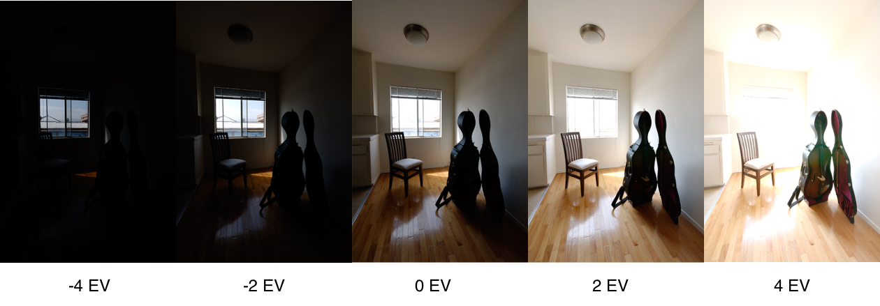
Hable’s example at varying EVs. The lowest EV captures the outside sky well, whereas the highest EV captures the cello details. (Note these EV values are relative to the original exposure)

In terms of the 1D exposure scale, by changing the EV, you shift your entire range over. At 0 EV, most of the room is in range. Decreasing the exposure by 4 stops shifts the range up: the bright outside sky is now well within range but now most of the room is underexposed and clipped to black. Increasing the exposure 4 stops does the opposite, centering the range around the details in the cello, but then what was previously in range is above the limits of the camera range and becomes overexposed and blown out.

Increasing the exposure centers our range around darker areas of the scene, shifting our range to the left on the EV scale. Some areas that were previously in the range will now be blown out. Decreasing exposure does the opposite.

As an example of what we’ve talked about so far, high dynamic range images are constructed by taking different exposures of the same scene and combining them into a file with a much higher dynamic range than a camera can capture in a single take or a display can show.

Tonemapping

Adjusting exposure didn’t solve everything as you can probably tell. With the high dynamic range example scene, we still had clipping no matter what we centered our range on (though we were able to focus it on different subjects). This is unfortunately inevitable, but it would be nice if we could use our range a bit more effectively.

Ideally, we would like our shadows and highlights to tail off to their limits rather than suddenly clip when outside our range. Instead of a direct or linear mapping from input to output range, we might also want to squeeze more EVs into the highlights and shadows, to preserve some detail. How we map the range is called tonemapping.

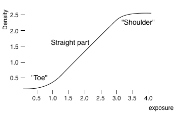
In film photography, we don’t have much control, but a film’s characteristic response curve is a built-in tonemapping. Essentially film reacts more slowly towards the extremes, so the shadows and highlights fall off gently and keep detail.

Characteristic film response curve

An example characteristic curve for film. At the “toe” and “shoulder” the film tails off to the limits.

With graphics, we have more control than physical cameras because we’re dealing with the unclamped light intensities from HDR rendering. We have all the lighting information from the HDR scene, so we can choose to map this information to our final display range however we want. A common approach though is to create an s-curve similar to camera film (referred to as filmic tonemapping).

Examples of tonemapping from Mirror’s Edge: Catalyst, show in Fabien Christen’s GDC 2016 talk. The first shows Linear tonemapping to filmic, and the second shows filmic to a more extreme tonemapping.

In these examples from Fabien Christen’s talk on Mirror’s Edge: Catalyst, you can see how the tonemapping reduces the blowout in the highlights, and gives better distinction between the specular reflections and the diffuse. He also points out after tonemapping the image will look a bit flat, but the point here is to give the range and detail you need for grading and other post processing.

Finally in the 1D scale, this can be visualized as a mapping (of tones!) from the input range to the limited output range.

Seena Burns

DEVLOG

Oct 16 - Dynamic Range, Exposure And Tonemapping

Dynamic Range

Exposure

Tonemapping

Further Reading